← Back to Main Page ... Go to Next Page (Background)
Introduction
Causal representation learning discovers causal relationships underlying data rather than statistical associations. At its core, causal representation learning seeks to identify high-level causal variables from low-level observations, bridging the gap between statistical pattern recognition and causal reasoning. Learning these causal variables offers transformative potential for artificial intelligence systems that can reason about cause and effect.

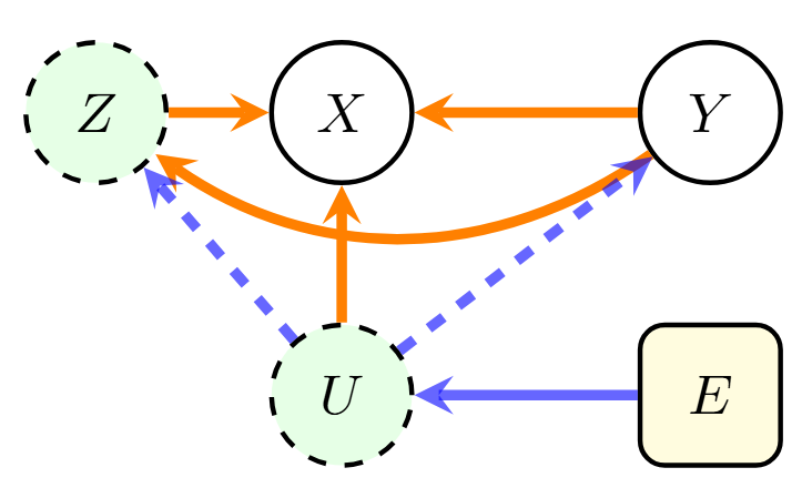
Figure 1: Anti-Causal Diagram
This diagram illustrates the Anti-Causal setting, showing causal (orange), spurious (blue), and confounding (dashed blue) dependencies. The nodes are $X$ (Observable variables), $Y$ (Causal variable/target), $Z$ (Unmeasured intermediary/latent), $U$ (Confounder/latent), and $E$ (Environment variable). Orange arrows represent direct paths to $X$, and blue arrows represent confounding effects. The core anti-causal structure is $Y \rightarrow X \leftarrow E$ mediated by latent factors $Z$ and $U$.
A particularly challenging yet promising domain is learning representations in the anti-causal setting, where the causal direction is reversed from traditional prediction tasks. Figure 1 diagrams the anti-causal setting, where $Y$ (target) is the causal variable, $X$ (observation) the observable variables, $E$ (Environment) the environment variable introducing spurious correlations, $U$ is a confounder which affects both $X$ and $Y$, and $Z$ (latent variable) is an unmeasured intermediary. The orange arrows represent direct paths to the observed variables $X$, and blue arrows represent confounding effects.
Consider a disease diagnosis from chest X-rays across different hospitals. A disease ($Y$) causes observable symptoms and measurements ($X$), with the relationship represented as $Y \rightarrow X$. The confounding factors $U$ (e.g., age and sex) affect both disease and symptoms. Environmental factors $E$ (e.g., hospital-specific protocols) introduce spurious correlations by creating hospital-specific variations, forming the anti-causal structure $Y \rightarrow X \leftarrow E$. The orange arrows therefore depict the true disease-to-symptom mechanism ($Y \rightarrow X$), while the paths involving $E$ and $U$ introduce noise. This anti-causal structure requires specialized methods to disentangle causal mechanisms from environmental artifacts.
Early works formalized anti-causal learning and showed that traditional methods fail in this setting. Follow-up works can be categorized into three main approaches:
- Intervention-based causal learning that models causal effects through interventions;
- Structure-based causal methods explicitly models causal structures through Directed Acyclic Graphs (DAGs), requiring complete knowledge of the underlying Structural Causal Model (SCM);
- Invariant learning methods that seeks representations invariant across distributions.
Limitations of Existing Methods
However, existing methods face several critical limitations:
- First, intervention-based approaches assume perfect interventions—where intervened variables are completely disconnected from their causes—a restrictive assumption rarely satisfied in real-world scenarios.
- Second, structure-based methods' reliance on explicit structural dependencies through SCM poses significant hurdles when the underlying SCM is unknown.
- Third, distribution-invariant approaches' assumptions on independent and identically distributed data or known test distributions limit the methods' generalization capabilities.
Fundamentally, these limitations arise because the single-level representations learned by these methods cannot simultaneously capture the causal mechanism from $Y$ to $X$ while filtering spurious correlations from $E$ to $X$ in anti-causal structure.

Figure 2: ACIA: Anti-Causal Invariant Abstraction Framework
This framework outlines four steps:
- Input (Raw Data): Illustrates the anti-causal structure $Y \rightarrow X$ and $E \rightarrow X$.
- Theorem 3 (Causal Dynamics): Learns a Low-Level Representation $\phi_L: \mathcal{X} \rightarrow \mathcal{D}_{\mathcal{Z}_L}$, capturing anti-causal structure and environment variations.
- Theorem 4 (Causal Abstraction): Learns a High-Level Representation $\phi_H: \mathcal{D}_{\mathcal{Z}_L} \rightarrow \mathcal{D}_{\mathcal{Z}_H}$, distilling environment-invariant causal features.
- Output (Two-Level Optimization): The final function $f=\mathcal{C} \circ \phi_H \circ \phi_L$ is optimized with a min-max objective subject to a loss $\mathcal{L}$ and regularizers $R_1$ (Environment Independence) and $R_2$ (Causal Consistency).
Anti-Causal Invariant Abstraction (ACIA)
We develop Anti-Causal Invariant Abstraction (ACIA), a two-level representation learning method (Figure 2), to address above limitations. ACIA is inspired by recent causal representation learning studies and measure-theoretic causality.
Specifically, to address the first limitation, we introduce a generalized intervention model that accommodates both perfect and imperfect interventions via the designed interventional kernels. To address the second limitation, ACIA learns directly from raw input without requiring explicit SCM specification. To address the third limitation, we introduce environment-invariant regularizers that enable stable identification of invariant causal variables across environments.
All together, ACIA involves:
- Causal Dynamics to learn low-level representations directly from data—without requiring explicit DAGs/SCMs—that capture the anti-causal structure by encoding how labels generate observable features while preserving environment-specific variations. E.g., in medical diagnosis, this reflects how diseases ($Y$) manifest as symptoms and measurements ($X$) in X-ray images, encompassing both disease-related patterns and hospital-specific factors. The learnt low-level representations support reasoning under both perfect and imperfect interventions, enabled by the interventional kernels.
- Causal Abstraction to learn high-level representations that distill environment-invariant causal features from the low-level representations. These abstractions generalize across environments by discarding spurious environmental correlations while preserving label-relevant mechanisms. For example, this involves identifying patterns that are consistently associated with specific diseases regardless of the hospital environment.
- Theoretical Guarantees that establish convergence rates, out-of-distribution/domain generalization bounds, and environmental robustness for the learned representations.
We extensively evaluate ACIA on multiple synthetic and real-world datasets with perfect and imperfect interventions. For instance, our results demonstrate ACIA achieves almost perfect accuracy (e.g., 99\%) on widely-studied CMNIST and RMNIST synthetic datasets with perfect environment independence and intervention robustness, significantly outperforming SOTA baselines. Most notably, on the real-world Camelyon17 medical dataset, ACIA achieves 84.40\% accuracy—an 19\% improvement over the best baseline (65.5\% by LECI)—while maintaining competitive environment independence and low-level invariance metrics. These results validate our theoretical framework's ability to learn robust anti-causal representations across both synthetic and real-world settings, with particularly strong performance gains in scenarios with complex environmental variations.